Tools
The following tools are available:
- Free Edge
- Mass and COG Table
- Moment Shear Force
- Moment Ratio
- Weld Summation Tool
- Effective Plate Width
- Stress Gradient
- Brace Stress
- Brace Classification
- Rainflow Counting
- Interpolation Tool
- creates a text file with materials, properties, nodes and elements ids without the model data. The file is used to debug user problems without having the customer model.
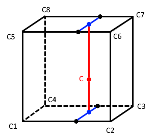
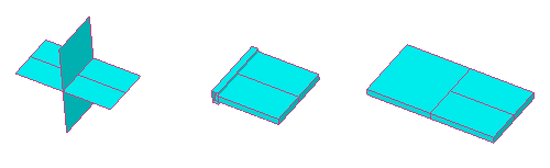
Free Edge
Free Edge Tool automatically finds free edges between the elements.
To open Free Edge execute from the ribbon.
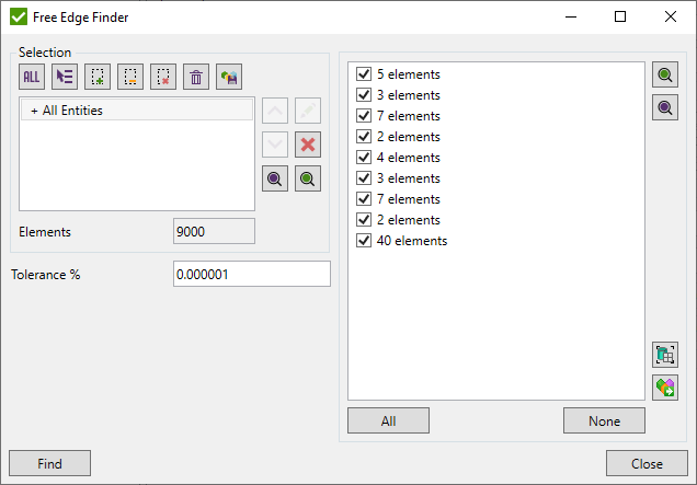
Press and the table will be filled with the groups of elements that have Free Edges;
Press to select all groups from the list and - to deselect;
 - display only groups of elements;
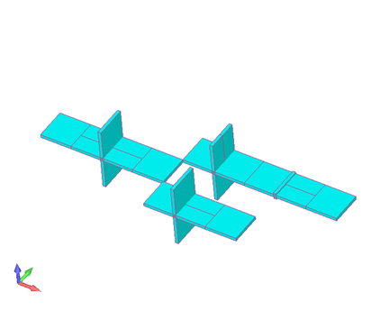
 - highlight the selected groups of elements;
 - export selected groups to Femap;
 - export selected groups to components.
Mass and COG Table
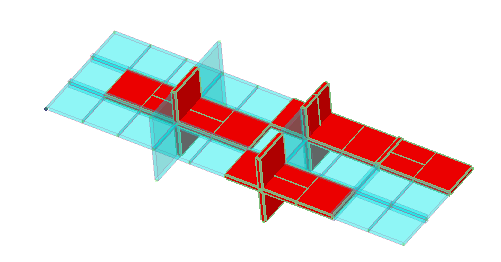
Mass and Center of Gravity Table is used to automatically calculate mass and center of gravity characteristics on the user-defined selections.
To add Mass and Center of Gravity execute from the ribbon.
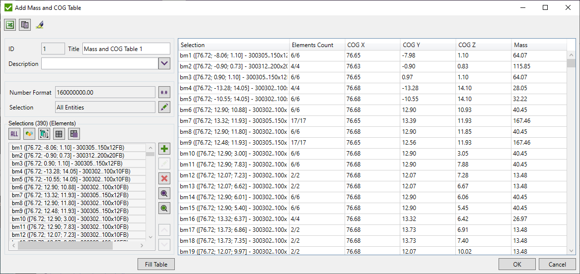
Selection - elements that will be intersected with the selections defined below;
Elements Count - first value is the amount of elements that were found on Selection. Second value is the total amount of elements that exist in the model;
COG X, Y, Z - coordinates of the center of gravity;
Mass - mass of the selection.
Note: Overall row is a Mass of all selections.
Selections can be defined using Selection List Control.
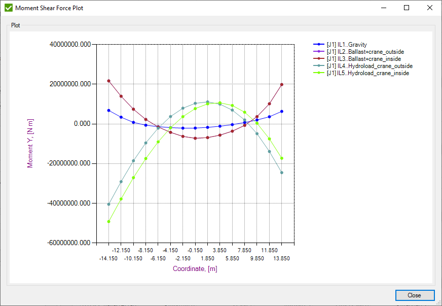
Moment Shear Force
In order to check the validity of a ship Moment Shear Force can be performed.
To add Moment Shear Force execute from the ribbon.
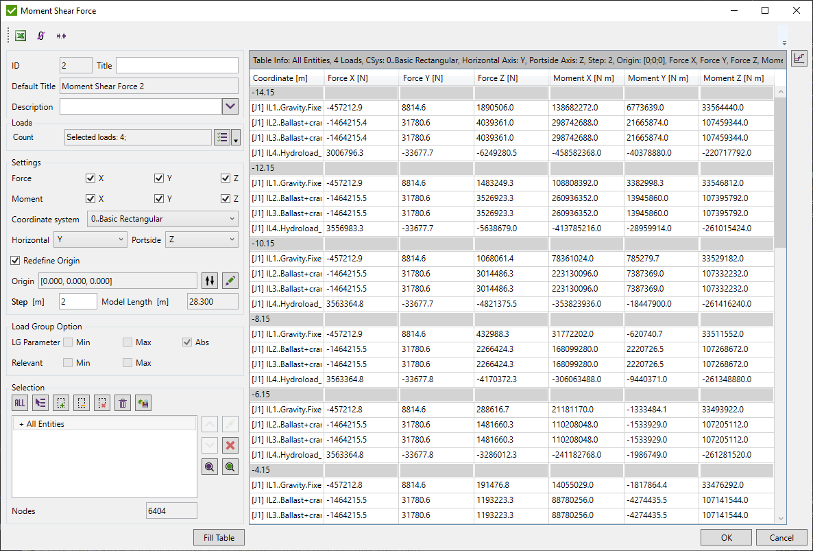
Select loads using Multiple Loads Selector.
Define selection using Selector Control.
Force/Moment X/Y/Z - select what Forces and Moments to display in the table;
Coordinate system - present results in the selected coordinate system;
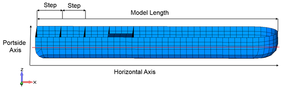
Horizontal - axis along the length of the model;
Model Length - defined automatically = Maximum - Minimum along the Horizontal axis;
Portside - axis along the height of the model (perpendicular to the Horizontal axis);
Step - model Length is divided by steps in a number of the locations where Forces and Moments will be calculated (N = Moment Length / Step).
By default, forces and moments are calculated around [0;0;0]. Selection option Redefine Origin and click  to select the location on the model. Press
  to set the origin to average coordinates from selection for all axes and min coordinate for the horizontal axis.
Sum of Forces and Moments are calculated based on Grid Point (Elemental-Nodal ENFO, ENMO) Forces/Moments. Pay attention that the results are included in the analysis.
For Load Group it is possible to show Min/Max/Abs values and also show loads from load group that contains min/max values (Relevant Min/Max).
Press to display the results.
 - select direction and display plot:
Moment Ratio
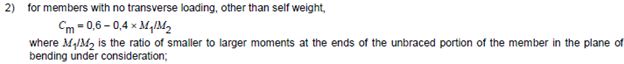
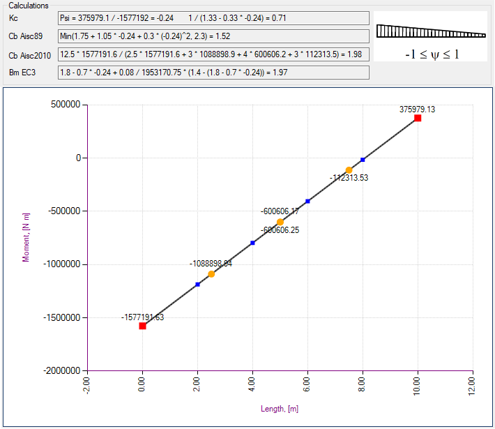
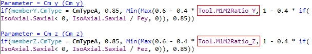
Moment Ratio calculates Kc and Bm factors (Eurocode3), Cb reduction factor (AISC), Cm - moment ratio on the ends of members found by Beam Member Finder.
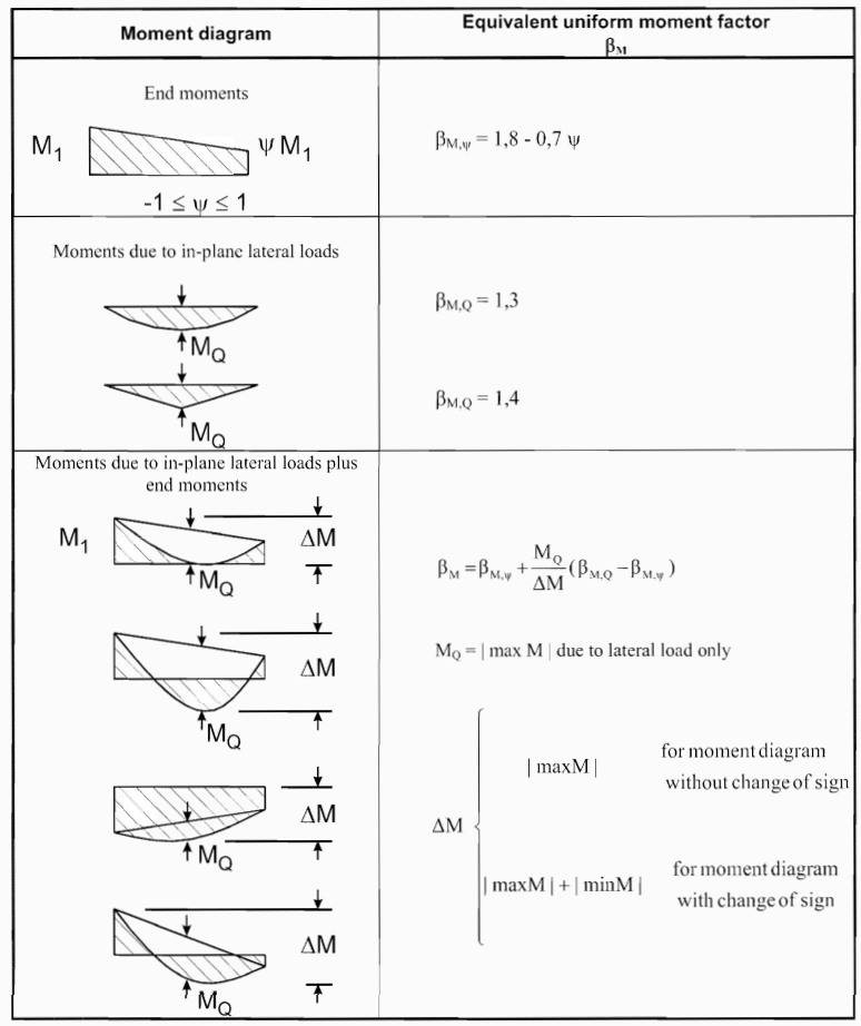
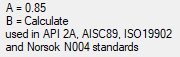
It is used in the moment reduction factors calculations in the following standards: API 2A RP (table D.3-1), ISO 19902 (table 13.5-1) and Norsok N004 (table 6-2):
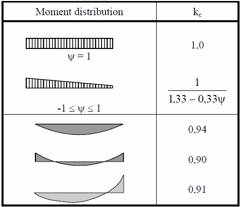
And moment reduction factors according to Eurocode3 (table 6.6):
Cb (Aisc2010) lateral-torsional buckling modification factor for AISC360-10 is calculated for the Moment Ratio Torsional Y and Z:
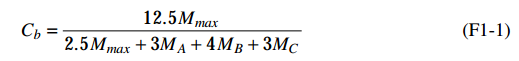
Cb lateral-torsional buckling modification factor for AISC ASD 89 (Section F1.3) is calculated for Moment Ratio Torsional Y and Z:

Bm Equivalent uniform moment factor for EN 1993-1-2:
Four moment ratio tools are created by default for length y, length z and length torsional members with Y/Z moment ratios. To edit the respective Moment Ratio execute from the ribbon.
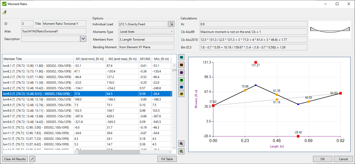
Moments Type:
M1(end min) and M2(end max) - the bending moment on the ends of the beam member;
M1/M2 - the moment ratio between the ends of the beam member;
Min/Max - the minimum/maximum bending moment over the full member;
Kc - the reduction factor according to Eurocode3, Part 1-1 Table 6.6;
Cb (Aisc89) - the lateral-torsional buckling modification factor according to AISC ASD 89;
Cb (Aisc2010) - the lateral-torsional buckling modification factor according to AISC360-10;
Bm (EC3 Fire Design) - Equivalent uniform moment factor according to Eurocode3, Part 1-2 Figure 4.2;
Select Load using Load Selector Control.
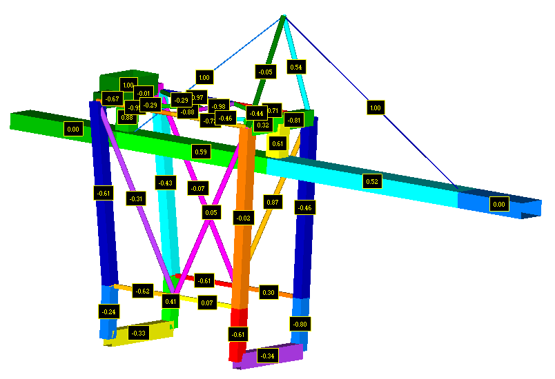
 - plot moment ratios (M1/M2) for the selected members;
 - plot ids for the selected members;
 - plot Cm Type for the selected members. Cm type can be changed in Beam Member Finder:
 - plot Kc factor;
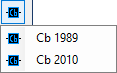 - plot Cb factor for AISC ASD 89 or AISC 360-10;
 - plot Bm factor for Eurocode3 Fire Design;
- highlight the selected beam members;
- preview only selected beam members.
For the selected member the bending moment diagram is displayed. End moments, Min/Max over the full member are shown with labels:
Example: Calculation of the reduction moment factors Cm according to ISO 19902:
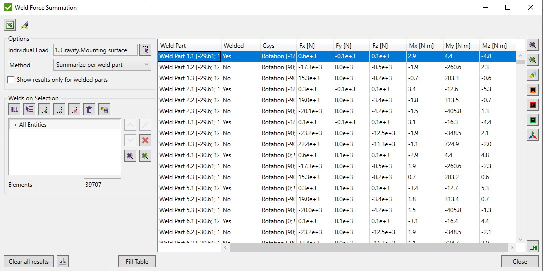
Weld Summation Tool
Weld Summation tool is used to summarize Grid Point Forces that will be used in Weld Checks to calculate the Weld Stresses.
Press  to automatically highlight a single selected weld/weld part from the list.
There are two methods available:
- Summarize per weld part - summarize forces at all welded nodes of the respective weld part. Mesh-independent and each weld part is treated as a structure;
- Summarize (Elemental-Nodal) - summarize forces at each welded node from respective weld part elements. Result depends on the mesh and the force distribution over the nodes;
Show results only for welded parts - display only welded parts of the welds in the table. The non-welded parts do not provide results in weld checks.
Select Load using Load Selector Control.
Press to display results.
Summarize per weld part
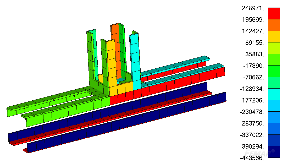
This method is used for the straight welds. Weld length and a coordinate system are taken from the Weld Finder Tool.
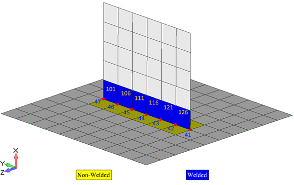
Forces are summarized over the weld nodes (41 - 47) using elements only from the respective weld part (101 - 126).
Weld part origin is used to calculate a moment arm for extra moments from the forces.
After forces are summarized, they are transformed into a weld part coordinate system.
Summarize (Elemental-Nodal)
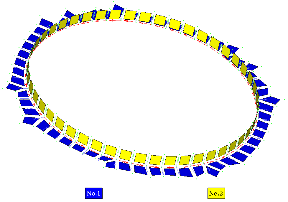
This method summarizes forces at each welded node from respective weld part elements. Besides, the weld length and a coordinate system are calculated for each weld node taking into account neighbor weld part elements.
Weld length is a sum of the half of the length of vector between adjacent weld nodes (L1 - L5 on the picture below):
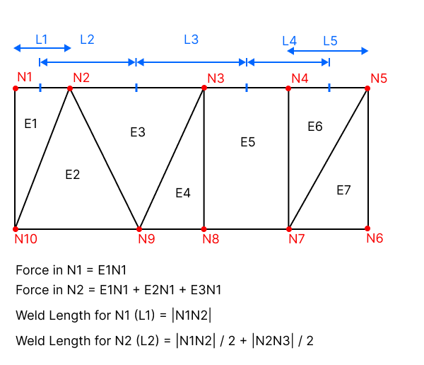
Note: For non-welded nodes, the result is taken from welded nodes by the following rules:
- For Element 1: FN10 = Average (FN1, FN2)
- For Element 2: FN10 = FN9 = FN2
- For Element 5: FN8 = FN3; FN7 = FN4
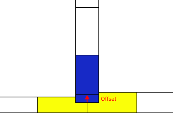
For each weld element, additional offsets and moments are computed individually, utilizing adjacent elements from weld parts positioned at perpendicular angles (within 90 degrees, with 5 degrees tolerance).
The offset is determined using half the average thickness of neighboring weld part elements:
 - open Weld Finder Tool to recognize welds;
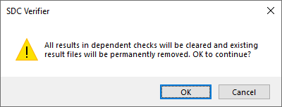
Press to recalculate forces. All results in weld checks will be cleared automatically after confirmation:
- highlight selected weld parts;
- preview selected weld parts;
 - display criteria plot for selected direction:
Note: Force and moments for the elemental method will show the absolute maximum value on the element from among its welded nodes.
- display colored weld plot with weld ids as labels;
 - display forces as labels for selected weld parts;
 - display moments as labels for selected weld parts;
Note: Forces and moments labels for the elemental method will display the values from all the welded nodes of the element.
 - draw coordinate systems based on selected Method. Per full weld, the method uses information from the Weld Finder Tool.
Elemental-Nodal method calculates a coordinate system at each node. Averaged vectors from the neighbor elements are used:
- draw coordinate systems based on selected Method. Per full weld, the method uses information from the Weld Finder Tool.
Elemental-Nodal method calculates a coordinate system at each node. Averaged vectors from the neighbor elements are used:
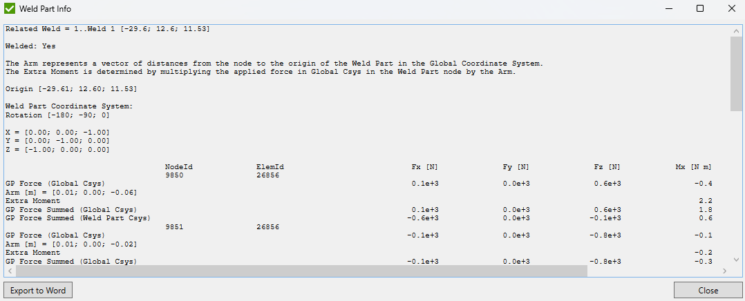
 -detailed information about single weld part, including results for each element/node.
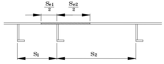
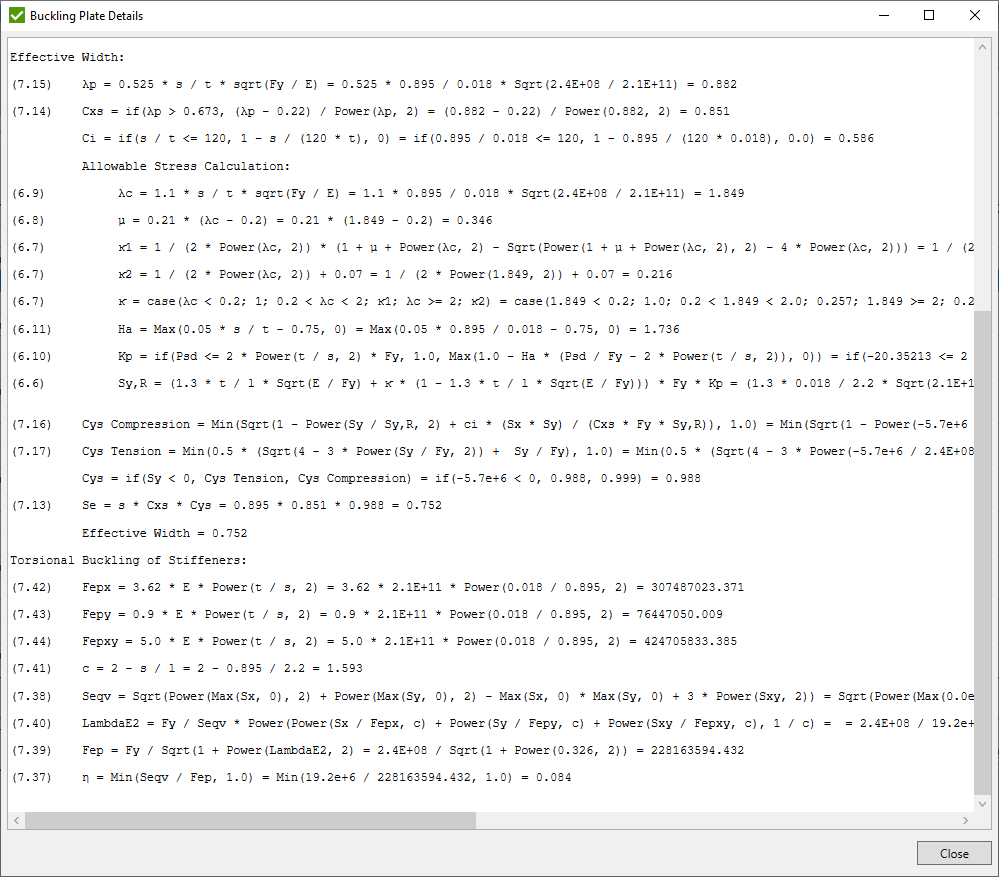
Effective Plate Width
Effective Plate Width - calculates effective plate width for a stiffener subjected to longitudinal, transverse and shear stress according to DNV-RP-C201 Buckling strength of plated structure, Chapter 7.3 Effective plate width. Also, it calculates η coefficient (formula 7.37) from chapter 7.5.2 Torsional buckling of stiffeners.
To edit Effective Plate Width execute from the ribbon:

Select Load using Load Selector Control and press . List of all sections with stiffeners and their related plates will be shown.
- highlight selected plates/stiffeners;
- preview selected plates/stiffeners;
It is possible to display plot with results as labels:
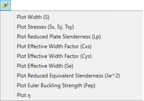
To see the details of the calculations select a single plate and press :
Stress Gradient
Related Stress Gradients - is calculated to reduce peak stresses at the defined points of the model.
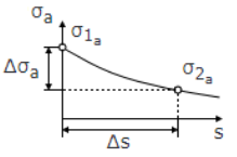
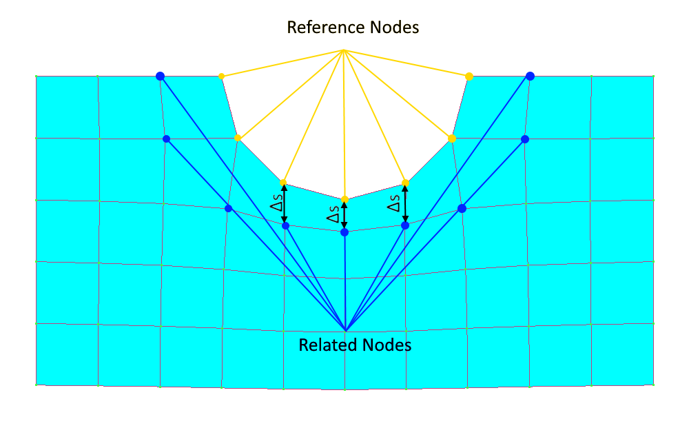
Calculations are based on normal and shear stress amplitudes at the reference point and point below the surface according to Equation 4.3.16 of Analytical Strength Assessment of Components in Mechanical Engineering, 5th Edition, 2003:
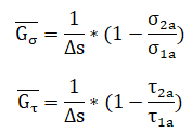 , where
σ1a, τ1a - stress amplitudes at the reference point;
σ2a, τ2a - stress amplitudes in a distance Δs;
Δs - the distance between the reference point and the neighboring point below the surface;
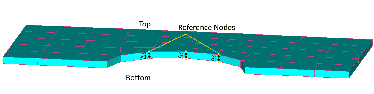
Note: Stress Gradient is calculated on free edge nodes of shell elements for their top and bottom points of interest.
To edit Stress Gradient execute from the ribbon.
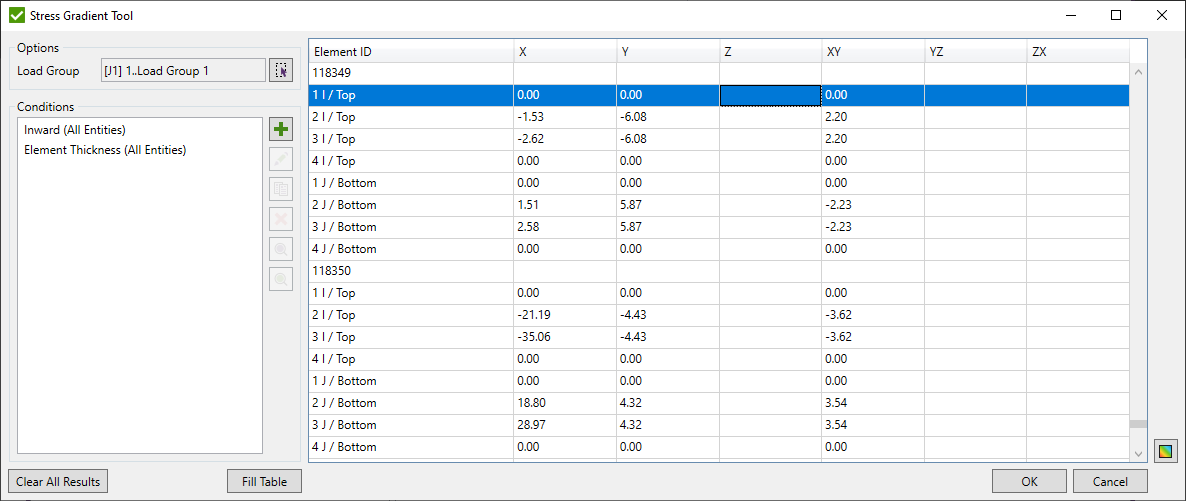
Select Load Group using Load Selector Control.
 -
-
- edit selected condition;
 - copy selected conditions;
 - remove selected conditions;
- highlight selected conditions on the model;
- preview selected conditions on the model;
 - plot stress gradients as contour plot for all calculated elements;
Define conditions and press to display results.
Stress Gradient Conditions
Stress Gradient is calculated for each point of interest (top and bottom) of all reference nodes. The condition can be added by the following types:
- select elements using Selector Control to find free edge nodes automatically (reference points) and take neighbor nodes (points below the reference point) from the selected elements to calculate stress gradient coefficient:
- select elements using Selector Control to find free edge nodes automatically (reference points) and take the opposite points of interest for each node (points below the reference point) from the selected elements to calculate stress gradient coefficient:
- pick reference/related elements and set points below the surface manually:
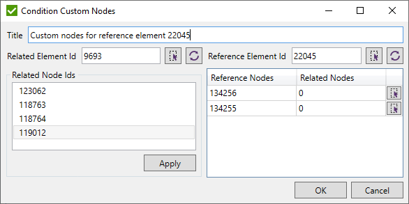
 - pick element/node from the model;
 - update the list of nodes of Related/Reference element;
 - apply selected related node to all selected reference nodes in the list;
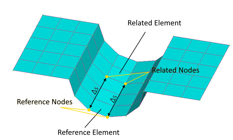
Related Element - stresses at the related nodes will be taken from this element. Pick element from the model or set manually;
Reference Element - a list of reference nodes will be recognized automatically from the free edges of the element. Stresses at the reference nodes will be taken from this element. Pick an element from the model or set manually;
Related Nodes - points below the surface to calculate the stress gradient;
Reference Nodes - reference points to calculate the stress gradient.
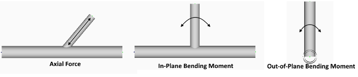
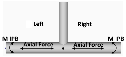
Brace Stress Tool
Brace Stress Tool is used to calculate axial, in-plane and out-of-plane bending stresses for braces and chord of connections recognized in Connection Finder. Calculations are based on axial force and bending moments, area and elastic section modulus of the cross section at the joint node.
To open Brace Stress Tool execute from the ribbon.
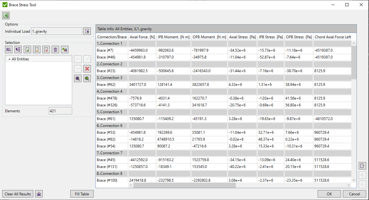
Select Load using Load Selector Control.
Define selection using Selector Control
- highlight the selected braces on the model;
- display only selected braces on the model;
 - export selected braces using Export Menu;
 - export the table data to Excel;
 - open Connection Finder tool.
Press to display info on the set parameters.
Press to clear results for all calculated loads.
Brace Classification Tool
Brace Classification Tool is used to calculate percentage of brace classification (K, TY, Cross) in the connection depending on what load is applied.
To open Brace Classification Tool execute from the ribbon.
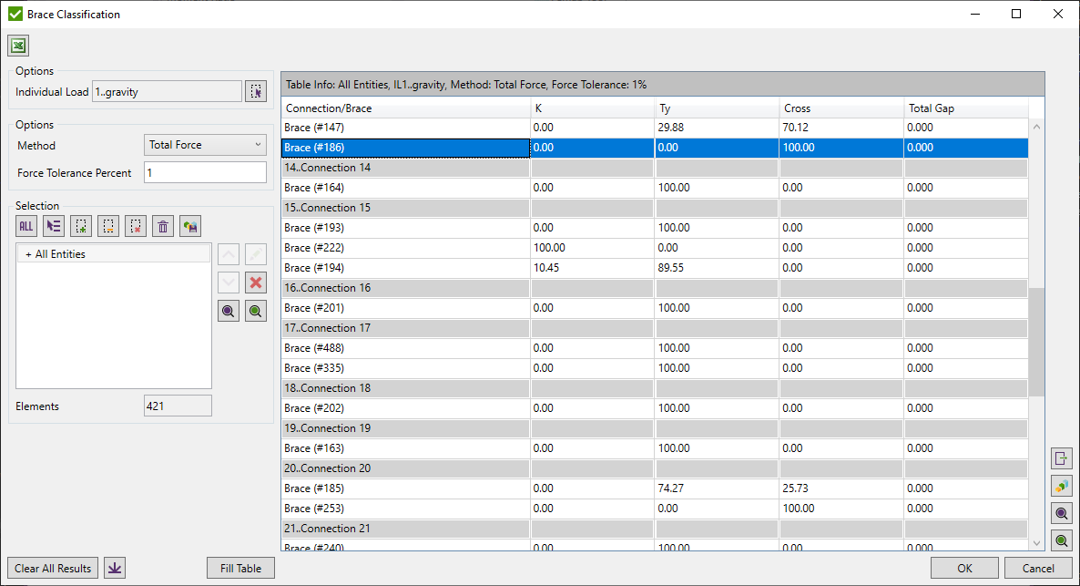
Select Load using Load Selector Control.
Define selection using Selector Control.
- highlight the selected braces on the model;
- display only selected braces on the model;
- export selected braces using Export Menu;
- export the table data to Excel;
- open Connection Finder tool.
Press to display info on the set parameters.
Press to clear results for all calculated loads.
Force Tolerance Percent - minimum percentage tolerance to check the tension and compression forces of all braces from one side of the chord (upper or lower) are balanced.
Method - calculate brace classification by one of the methods described below. Braces are classified into K, TY, and Cross (X) types. The order of recognition for all methods is the following: K -> Cross (X) -> TY.
K - tension and compression loads are balanced.
TY - tension or compression load goes as a shear force in a chord.
Cross (X) - Connection has to contain braces from both sides to check on cross joint.
Note: If the brace has zero force, the joint type for such brace is set to TY.
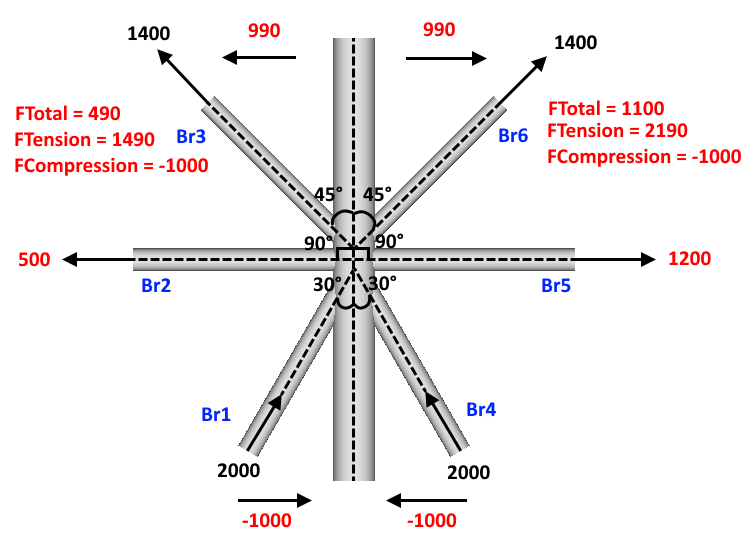
Total Force Method
Total Force Method is based on the summed axial forces of all braces from one side of the connection by checking if they are balanced.
Example:
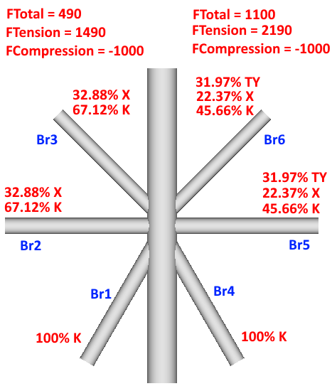
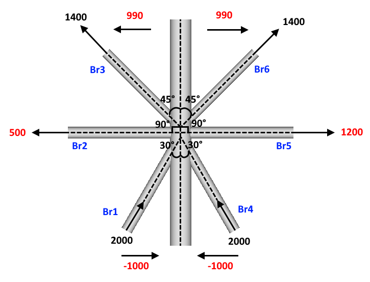
We have connection with 3 braces from one sided of the chord and 3 braces from other side of the chord with their initial forces. Calculations start from summarizing forces that are perpendicular to the chord at each side of the connection:
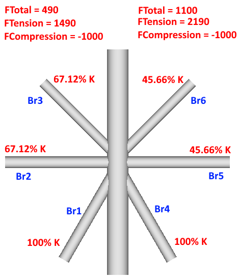
K calculations:
Algorithm checks if FTotal is tension (all compression braces are 100% K) or compression (all tension braces are 100% K) at each side of connection. Rest of the braces are calculated by the following formula: Min(|FTension|, |FCompression|) / Max (|FTension|, |FCompression|) * 100%.
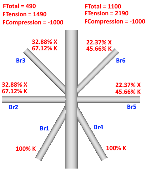
Cross (X) calculations:
If FTotal from both sides of chord are of the same sign - cross type is calculated. Braces from the side with the smaller FTotal are set to Cross (X) = 100% - K%. Braces from side with bigger force are calculated by formulas: FTotal / FCompression if brace is in compression and FTotal / FTension if brace is in tension. FTotal in this case is taken from the side with smaller value.
TY calculations:
After eliminating all the forces from all the braces that were used in K and Cross (X) calculations, all the forces that left on braces will provide shear in the chord and consequently are set to TY type.
Left-to-Right Method
Left-to-Right Method is based on comparing axial forces of the each pair of neighbor braces. Calculations start from the brace with the smallest angle to the chord to the last brace of one side of connection. If both edge braces have the same angles - default brace is chosen as a start brace.
Example:
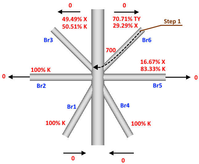
We have connection with 3 braces from one sided of the chord and 3 braces from other side of the chord with their initial forces. Calculations start from the braces from each side of the chord with the smallest angle to the chord (Br1 and Br4 respectively):
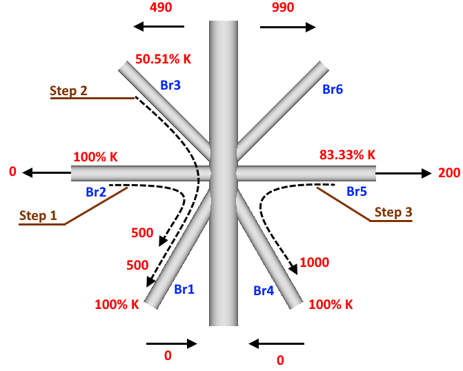
K calculations:
Algorithm checks all forces for each pair of braces from each side of connection on force balance:
Step 1. 500 force units are balanced between Br2 and Br1
Step 2. 500 force units are balanced between Br3 and Br1
Step3. 1000 force units are balanced between Br5 and Br4
Cross (X) calculations:
Forces are taken from the braces of the opposite sides of connection but the order of braces is kept, starting from the smallest angle:
Step 1. 200 force units from Br5 work together with 200 force units of Br3 in opposite directions from each other (both tension) that will not provide shear in the chord, consequently Br5 becomes Cross (X) type = 200 / 1200 * 100% = 16.17%;
Step 2. 290 force units from Br6 work together with 290 force units of Br3 in opposite directions from each other (both tension) that will not provide shear in the chord, consequently Br6 becomes Cross (X) type = 290 / 990 * 100% = 29.29%;
Step 3. 490 force units from total of 990 initial force units of Br3 becomes Cross (X) type = 490 / 990 * 100% = 49.49%;
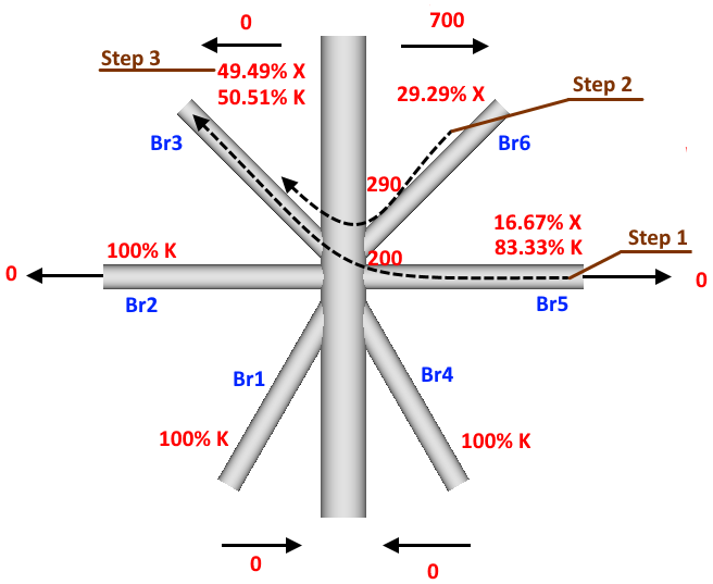
TY calculations:
After eliminating all the forces from all the braces that were used in K and Cross (X) calculations, all the forces that left on braces become shear will provide shear in the chord and consequently are set to TY type
Step 1. 700 force units of Br6 of total 990 initial force units become TY type = 700 / 990 * 100% = 70.71%; Or in other words: TY = 100% - K% - Cross (X)%: = 100% - 0% K - 29.29% Cross (X) = 70.71%;
Gap
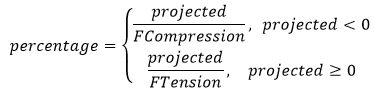
Gap is a minimum distance between two differently loaded braces (tension and compression, or K type) measured on a shell of the chord. It is possible that brace can have two or more gaps to considerate, in this case Total Gap parameter is a sum of all gaps multiplied on percentage of each that depends on the percentage of the taken load:
Projected - brace axial force that is perpendicular to the chord;
FTension - sum of all tensile projected axial forces;
FCompression - sum of all compressive projected forces.
Example of gaps:
Rainflow Counting
Rainflow Counting method is used to determine the number of fatigue cycles that is based on a load-time history. It is used in the analysis of fatigue data in order to reduce a spectrum of varying stresses into a set of simple stress reversals. This simplification allows the number of cycles until failure of a component to be determined for each rainflow cycle using either Miner's rule to calculate the fatigue damage, or in a crack growth equation to calculate the crack increments.
To open Rainflow Counting Tool execute from the ribbon.
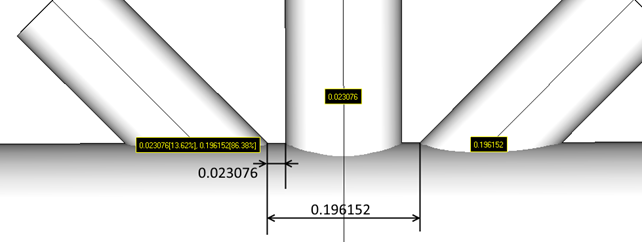
Options:
Settings:
Note: Load History will be automatically applied for a selected Load Group.
Hysteresis Gate Percent - ignore stress ranges that are less or equal than the percentage from maximum stress range;
Actual Hysteresis Gate - ignore stress ranges that are less or equal than the actual stress range value. Should be set in stress units;
Number of Bins - each bin is a fixed stress range. Number of bins split maximum stress range of a load-time history into a set of smaller stress ranges. The measured data points are mapped to the centers of their bin, which enables counting procedures;
Note: more number of bins is set - more accurate algorithm is, but calculation time is increased;
Half Cycle Calculation - filtering of initial stresses are performed only from Left to Right (Valley-to-Peak), Right to Left (Peak-to-Valley) or for Both;
LG Parameter - used in case if Load Group contains in a history another Load Group. Minimum, Maximum or Absolute Maximum result can be used in calculations;
Selection - select part of the model to be calculated by the tool using Selector Control;
Rainflow Counting consist of 4 main steps:
1. Peak-Valley Filtering.
Peak-Valley filtering removes all the intermediate load-time history results that are between all Peak and Valley pairs in order to get only minimum and maximum values of a cycle that are important for fatigue calculations:
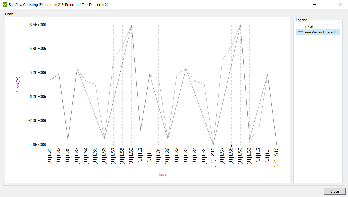
Initial (gray line) is the original load-time history of all the loads included in Load Group. Peak-Valley Filtering (dark gray line) is a filtered load-time history with excluded intermediate data points. Peak-Valley load-time history is used in further calculations.
2. Hysteresis Filtering.
Hysteresis filtering removes small stress ranges obtained after Peak-Valley filtering that have a negligible influence on a damage:

Peak-Valley (dark gray line) data is obtained from Step 1. Hysteresis Filtering (black line) is a filtered load-time history that excludes stress ranges that are smaller than the gate (percentage or actual value defined in the settings). Hysteresis load-time history is used in further calculations.
3. Binning
Binning splits the min/max stress range to the number of bins defined in the settings. Each bin represents a fixed stress range. Hysteresis load-time history data points are moved to the centers of the respective bins, which enables counting procedures.
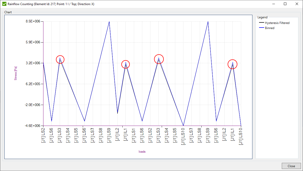
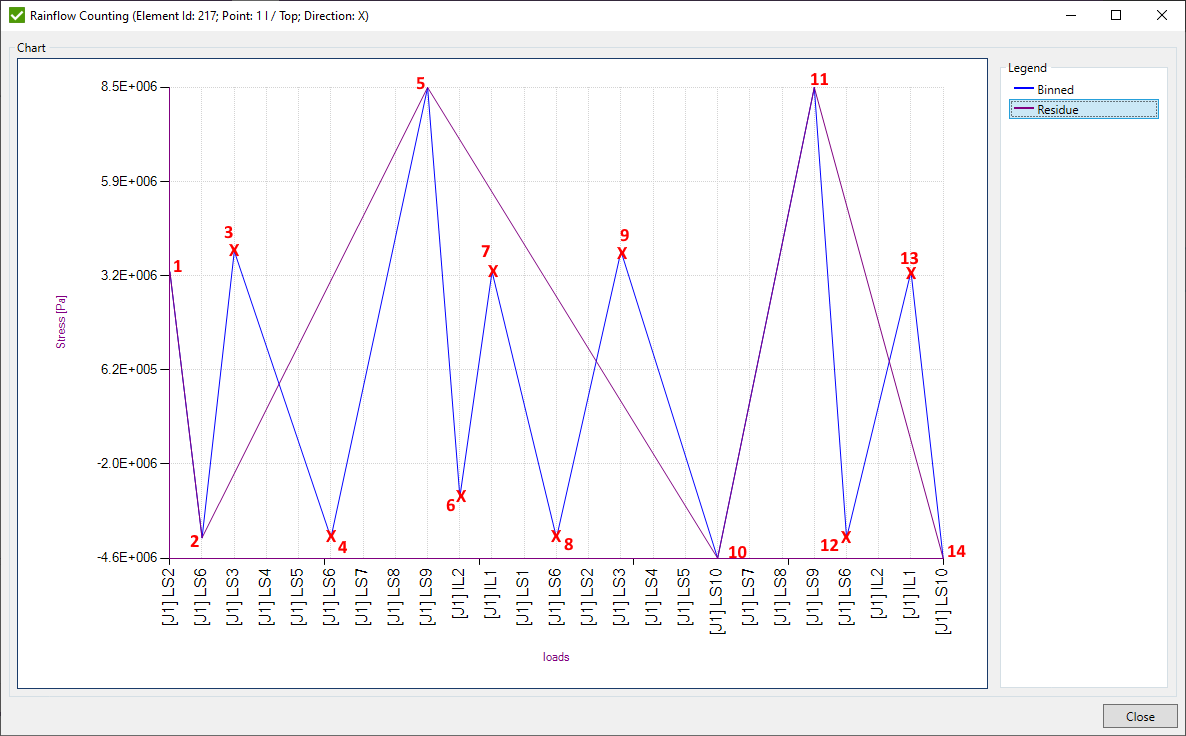
Hysteresis Filtering (black line) data is obtained from the Step 2. Binned (blue line) is a modified data after placing data to the centers of respective bins. Binned load-time history is used in further calculations.
4.a. Half Cycle Method
Half Cycle Method also known as Pagoda roof method counts half the cycle for each stress between its start and termination. Counting can be done for both Valley-to-Peak (Left-to-Right) and Peak-to-Valley (Right-to-Left) or for any of them that depends on the selected Half Cycle Calculation option.
Green (Peak-to-Valley) and red (Valley-to-Peak) lines on the picture below represents the counting path:
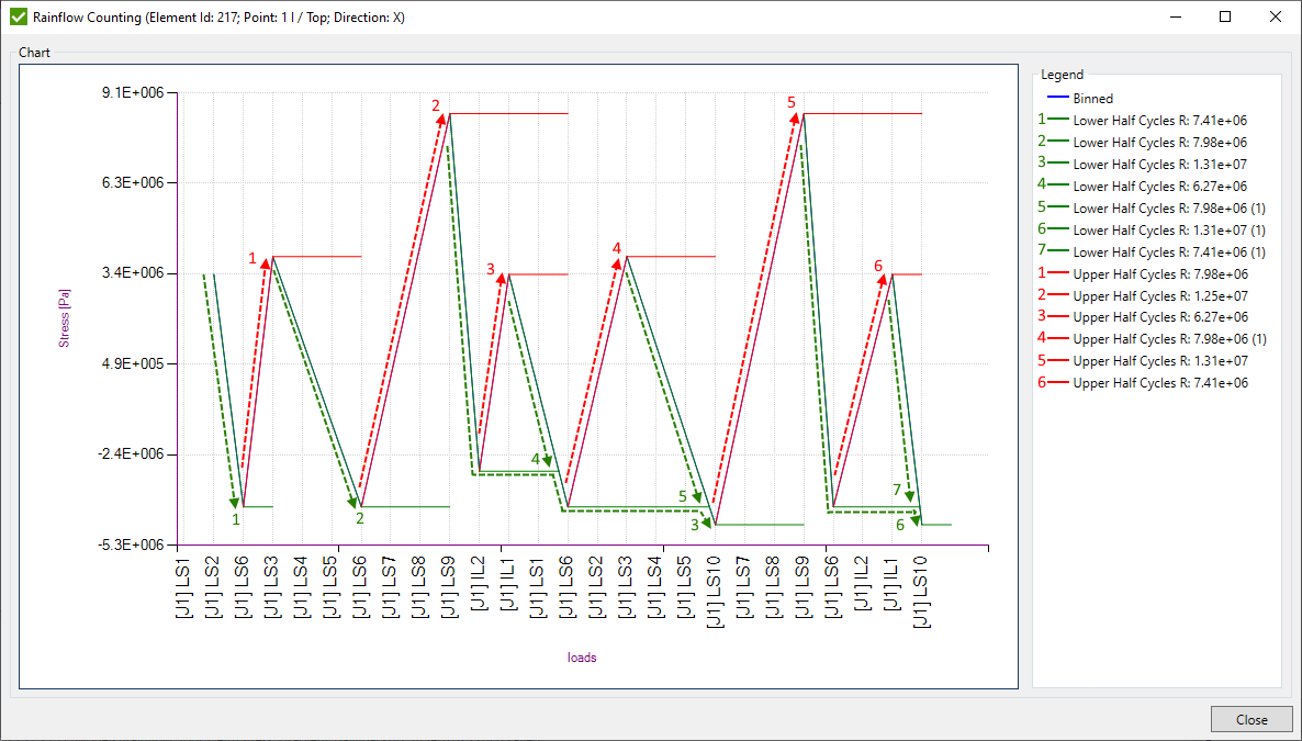
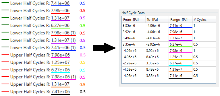
All the obtained stress ranges are gathered into the table and each occurred range is set 0.5 cycle. Afterwards all similar cycles are summarized that results in the Half Cycle Data table:
4.b. Four Point Method
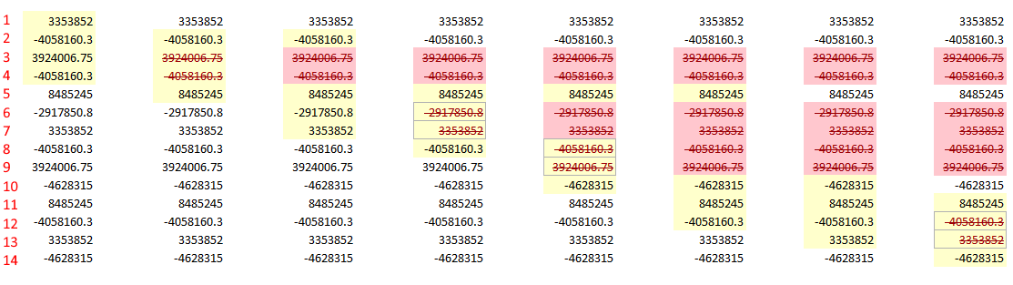
This method evaluates each set of 4 data points A-B-C-D of the binned data in turn to determine residual stresses and a rainflow matrix with number of cycles. Algorithm compares the stress ranges of points A-D and B-C and sets 1 cycle for the range of results using a stress value at point B (from) and point C (to) only if A-D >= B-C.
Numbered data points and each set of 4 points is checked. Points that are currently checked are highlighted in cream color. Points that are eliminated are crossed out and they provide a counted cycle. Rest of the points represent a Residual Stress and are included with the cycles. A cycle is counted if inner stress range (B-C) <= to outer stress range (A-D) and the points comprising the inner stress range are bounded by the outer
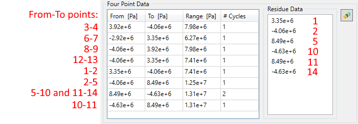
The Four Point Data includes eliminated and residue stress points that form ranges:
Matrix of calculated cycles is displayed on the graph:
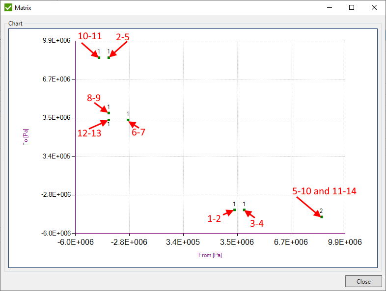
Note: cycles with equal from - to ranges are summarized.
Press to finish edit rainflow counting tool. Confirmation message of clearing results for checks that use rainflow counting will appear:
![]()
Interpolation Tool
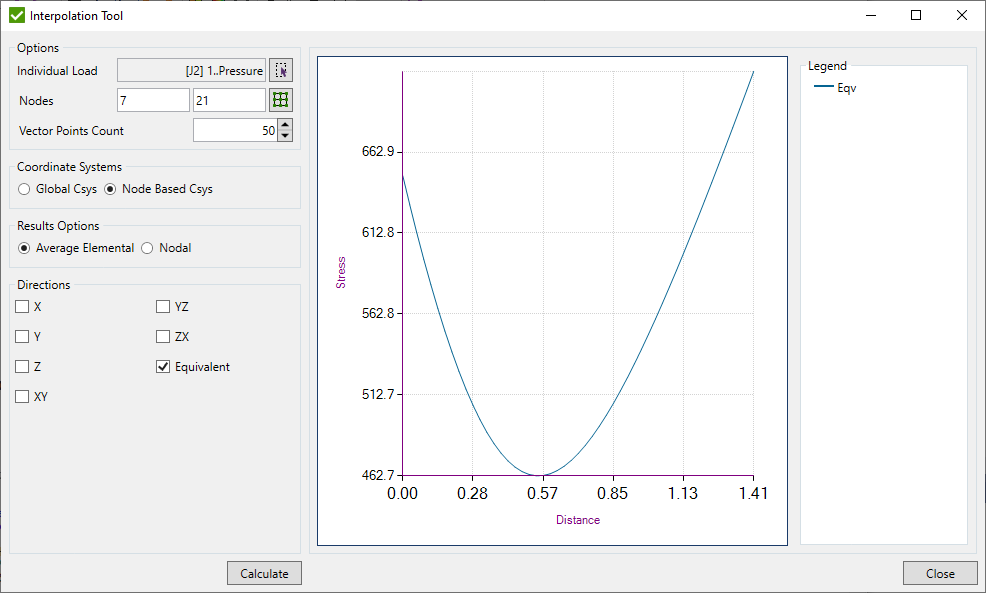
Interpolation Tool allows to display stress variation along the selected line between two mesh nodes.
To open Interpolation Tool execute from the ribbon.
Interpolation can be performed over selected Individual Load or Load Set.
Nodes - select nodes to define interpolation line;
Vector Points Count - set number of points between the selected nodes where stresses will be interpolated to display more detailed graph.
Coordinate Systems - transform stresses to the Global Csys or Node Based Csys before interpolating results. Node Based Csys is calculated by the following rules:
- X Direction - vector between selected nodes;
- Y Direction - rejection vector of X Direction and Global X Direction. If X Direction and Global X Direction are collinear, Global Y Direction is used;
- Z Direction - cross product vector of X Direction and Y Direction;
Results Options - use averaged stresses from neighbor elements at respective point of interest or corner stresses of the element to get the result at the interpolation point;
Note:Averaging is performed for currently calculated element using results from the connected elements at the element corner nodes. If type of current element is shell and line or solid element is connected - half of result of line or solid element will be added to the top and half to the bottom result of the shell element at the corner node.
Directions - list of directions that will be displayed on the graph;
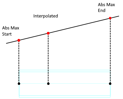
Note: For line elements point result will be displayed only if interpolation point is located on the line between start and end node of the line element. Result is a Linear Interpolation between absolute maximum results at both ends of the line element.
Note: Shell elements are treated as 3D element using the element thickness. Result is a Trilinear Interpolation between the top/bottom corner results of the element.