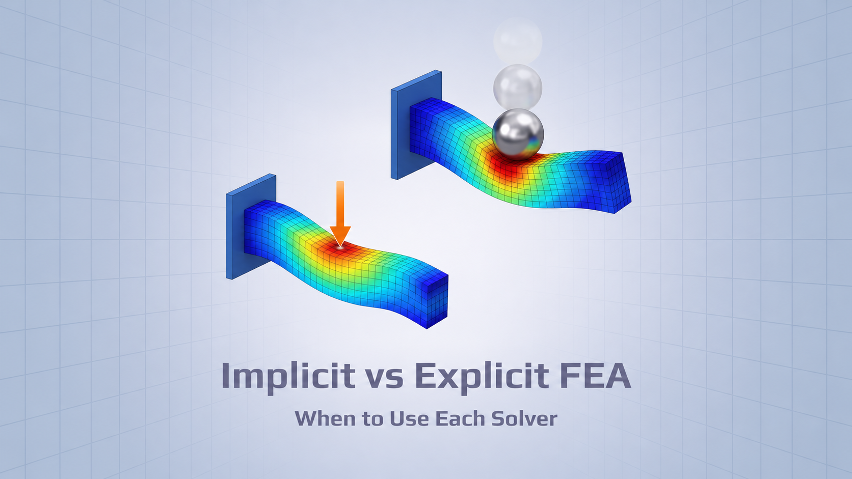
The choice between implicit and explicit finite element analysis affects how a simulation is solved, how much computational effort it requires, and which types of structural behavior it can follow efficiently. It is not simply a choice between static and dynamic analysis.
Implicit methods are commonly used for static loads and other problems where the solver can reach equilibrium reliably. Explicit methods are often better suited to short events such as impact or crash, especially when contact conditions change rapidly. Both methods can handle nonlinear behavior, and neither is limited to just one class of problems.
The useful distinction is how each method advances the solution. Once that is clear, the choice of solver becomes easier to connect to the actual engineering problem.
Go beyond the solver result
Already running explicit LS-DYNA analyses in Ansys Mechanical? SDC for Ansys lets you use those results for applicable strength, buckling, fatigue, and bolt checks — without rebuilding the verification workflow manually.
The Main Difference Between Implicit and Explicit FEA
An implicit solver works toward equilibrium at each load or time increment. In nonlinear analysis, it may need several iterations to correct the solution until the equilibrium criteria are met. This takes computational effort, but it often allows the solver to use comparatively large increments. If contact changes abruptly or the structure becomes unstable, those iterations can become difficult to converge.
An explicit solver takes another approach. It advances the response using known information from the current and previous time increments, without performing nonlinear equilibrium iterations at each step. Each increment is relatively inexpensive. The drawback is that the time step must remain below the numerical stability limit, which can be extremely small. A few small elements may even govern the time step for the whole model.
The overall cost depends on the problem. An implicit analysis may need fewer, more expensive increments; an explicit analysis may need a very large number of inexpensive ones. Both methods also need enough time resolution to capture the physical response accurately.
Characteristic
Implicit FEA
Explicit FEA
Solution approach
Solves coupled equations at each increment; nonlinear problems usually require equilibrium iterations
Advances through direct time integration without equilibrium iterations at each step
Main numerical constraint
Convergence and accuracy
Stable time step and accuracy
Time increments
Often relatively large
Usually very small
Computational cost
Higher cost per increment, often fewer increments
Lower cost per increment, potentially many more increments
Often suited to
Static and quasi-static loads; gradual contact; longer-duration dynamics
Impact, crash, drop tests, rapidly changing contact, and some failure problems
When to Use Implicit Analysis
Implicit FEA is usually a good starting point when the structure is loaded gradually and the main objective is to determine its equilibrium response. Common examples include equipment frames, steel supports, bolted assemblies, pressure loading, and operational load cases. Implicit dynamics can also be efficient for longer-duration responses that do not require very small time steps.
Consider a support frame carrying equipment and operational loads. A static implicit analysis can calculate stresses, displacements, and member forces without simulating the entire loading process in physical time. Those results may then be used for applicable strength or code-based buckling checks. This is different from simulating the frame’s actual buckling or collapse behavior.
An implicit solver can also handle nonlinear materials, large deformation, and contact. The difficulty is not the presence of nonlinearity itself, but whether the solver can follow the changing response and reach equilibrium at each increment.
When to Use Explicit Analysis
Explicit FEA is commonly selected when inertia and short physical time scales matter. Typical cases include impact, drop tests, collision, crash, and repeated or rapidly changing contact. It can also be useful for progressive fracture or element erosion, where implicit equilibrium iterations may become impractical.
A drop test illustrates the difference. At impact, contact forces change quickly, stress waves travel through the structure, and local plastic deformation or rebound may occur. Implicit dynamics can represent the event, but capturing it accurately may already require very small time increments. In that situation, the ability of an implicit method to take larger stable increments offers little benefit, while each increment remains more expensive.
Explicit analysis still requires careful checking. A completed simulation is not proof that the result is correct: mesh sensitivity, contact behavior, element distortion, hourglassing, and energy balance can all affect the answer.
When Either Solver Can Work
Many structural problems sit between the obvious static and impact cases. Large deformation, for example, does not automatically require explicit analysis. Both methods can handle large displacements and rotations. What matters more is whether deformation is accompanied by severe contact, instability, or failure, and whether the implicit solution remains practical.
Nor is every convergence problem a reason to change solvers. If an implicit analysis struggles near buckling or snap-through, smaller increments, displacement control, arc-length methods, or another suitable nonlinear procedure may be the better response. A code-based buckling check should not be confused with simulating instability or collapse.
Contact needs the same judgment. Gradual contact often works efficiently with implicit analysis. Repeated impact, self-contact, separation and re-contact, or rapidly changing contact regions may favor explicit integration.
Can Explicit Analysis Be Used for Quasi-Static Problems?
Yes. Explicit solvers are sometimes used for slowly applied loads, forming, or severe contact problems that are difficult to solve implicitly. The challenge is that a physically slow event can require an impractically large number of explicit time increments. Engineers may shorten the loading duration or use mass scaling to reduce runtime.
Both techniques can affect the result. Faster loading may introduce inertia or change the response of a rate-sensitive material. Mass scaling increases the stable time increment by adding mass, but it also changes inertia. Neither should be treated as a harmless solver setting.
For a quasi-static explicit result, the engineer should check more than the final deformed shape. Useful checks include:
Comparing the response with a slower-loading or reduced-mass-scaling run.
Reviewing kinetic and internal energy, including whether local regions show significant dynamic effects.
Checking force–displacement histories, reactions, and unwanted oscillations.
Monitoring hourglass, contact, and other numerical energies where relevant.
A favorable kinetic-to-internal-energy ratio is useful evidence, but it does not, by itself, establish that the simulation is quasi-static.
Implicit vs Explicit FEA: Decision Guide
These are starting points rather than fixed rules. The final choice depends on the duration of the event, contact and material behavior, numerical controls, and the results the engineer needs.
Engineering problem
Likely starting point
Reason
Linear or nonlinear static structure
Implicit
Efficient equilibrium solution when convergence is manageable
Gradually changing contact or bolted assembly
Usually implicit
Contact and loading can be followed incrementally
Long-duration, lower-frequency dynamics
Often implicit dynamics
Larger accurate time increments may reduce cost
Drop, crash, or short-duration impact
Usually explicit
Rapid contact and stress-wave response require fine time resolution
Repeated impact or rapidly changing contact
Often explicit
Avoids difficult equilibrium iterations
Progressive fracture or element erosion
Often explicit
Can follow rapidly evolving failure where implicit iterations struggle
Large deformation without severe contact or instability
Depends
Large deformation alone does not decide the solver
Static snap-through or postbuckling response
Implicit with suitable controls may be preferred
Displacement control or an arc-length procedure may follow the equilibrium path
Quasi-static forming with severe contact
Depends
Explicit may be practical, but loading rate, inertia, and mass scaling need checking
From LS-DYNA Results to Engineering Verification
Selecting the solution method is one engineering decision. Determining whether the calculated response meets the applicable design criteria is another.
SDC for Ansys works with analysis results available in Ansys Mechanical; it does not perform the explicit LS-DYNA solution itself. It supports results from explicit LS-DYNA analyses set up and solved through the LS-DYNA system in Ansys Mechanical, with Ansys 2023 R2 or newer. The documented scope includes applicable strength, fatigue, bolt, and buckling verification on those results.
The output interval matters. An explicit solver may calculate far more increments than it stores as result states. If a peak occurs between saved states, downstream verification may not capture it. Output should therefore be planned around the quantities that need to be evaluated.
The engineering check must also fit the event. A single impact is not automatically a fatigue spectrum, and a code-based buckling check is not the same as simulating collapse. The result quantities, selected time states, and assumptions of the relevant standard still determine what can be verified.
Turn LS-DYNA results into engineering verification
Solver results describe how a structure responds. SDC for Ansys helps engineers evaluate applicable LS-DYNA results against design criteria and prepare structured verification reports.
Yes. LS-DYNA supports both implicit and explicit solution methods for static and dynamic applications. The SDC for Ansys workflow described here refers specifically to supported explicit LS-DYNA results through Ansys Mechanical.
Can implicit and explicit methods be used in the same workflow?
Yes. An implicit preload may be followed by an explicit impact, or an explicit forming stage by an implicit springback calculation. The exact procedure depends on the solver and the state variables that must be carried between stages.
Is explicit FEA always faster?
No. An explicit time increment is generally less expensive, but an analysis may need a very large number of increments. For slow or long-duration problems, implicit analysis can be more efficient. Explicit often has the advantage for short events that already require fine time resolution.